Luận án Giải pháp học thích ứng trên nền tảng mạng học sâu ứng dụng nhận dạng đối tượng tham gia giao thông

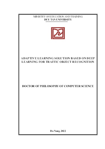
table frames) ( 
With each image, the CNN will extract the rich features, which are pedestrian 
postures, roadways, roadsides and positions of pedestrians on road, figure 2.5. The 
rich features extracted will be used for training SVM classifier model. 
a) Input image. 
b) Rich features simulation. 
Figure 2.4 Input images and simulate rich features of image 
 32 
. 
 In CNN model, many feature layers can be extracted such as convolution 
layer or full connected layer but the more advantageous layer is layer 19 (fc7 – 4096 
fully connected layer) – the one right before the classification layer. 
Literally, in cases of object recognition such as animals, things and vehicles, 
the rate of recognizing object is higher (90% to 100%). In case of predicting the 
action of pedestrians, the features of input images focus on not only a specific 
object but also others such as vehicles, buildings, trees, and things around roadsides 
as shown in Figure 2.5. 
Figure 2.5 Influence of other objects on the road on pedestrian movement prediction 
In this regard, in term of accuracy, ACF algorithm is used to detect 
pedestrians before extracting ROI, classifying and predicting the action of 
pedestrians. 
2.2.1.2 Pedestrian action prediction 
Pedestrian detection by ACF. ACF classification model, specified as 'inria-
100x41' or 'caltech-50x21', is person detection. The 'inria-100x41' model was 
trained using the INRIA Person data set. The 'caltech-50x21' model was trained 
using the Caltech Pedestrian dataset. The ‘inria-100x41’ model (default) is 
proposed in ACF. In ACF algorithm, detection scores value - confidence value - 
return an M-by-1 vector of classification scores in the range of [0..1]. When a 
pedestrian is detected, a bounding box will appear. The scores on top of bounding 
box are confidence value (by percentage). Larger score values indicate higher 
accuracy in the detection. In some complex images, the ACF algorithm sometimes 
 33 
recognizes errors. During the real-time experimental process, the score value 0.25 is 
proposed to avoid error-recognizing cases. For example, if the score value is 0.1, the 
result will not be accurate in some cases (Figure 2.7 (a)) and if the score value is 
0.25, the result will be of higher accuracy (Figure 2.7 (b)). 
Figure 2.6 Example input image for recognition 
a) b) 
Figure 2.7 Pedestrian detection with scores = 0.1 (a) and scores = 0.25 (b) 
In particular, when the AV moves on the roads, there are some cases in 
which so many pedestrians appear in one frame of the video. Therefore, to ensure 
the accuracy, it is considered that a frame be extracted into many separate frames to 
be easily recognized in each case. The region extracted is called ROI (Figure 2.8). 
Also, in real-time, the image received from AV is in big size and contains a lot of 
irrelevant data. Hence, extracting ROI of image at a certain scale, which removes 
irrelevant objects around, is necessary for each pedestrian detected. Extracting ROI 
of image helps the CNN model extract the exact features and reduce the error rate in 
the process of action recognition and classification of the SVM. The size of ROI is 
 34 
proposed as follows: 
Supposing that H and W are height and width of the rectangle covering 
pedestrian object; x and y are the coordinates of the top left of rectangle and Width 
and Height are the size of input image, the values x1, y1, W1, H1 describe the size 
of ROI which are defined as follow: 
( )
( )
1 1.5
1 – 
1 3
1 2
 1 1 
 1 1 
x x H
y y W
W W H
H H W
if W Width thenW Width
if H Height then H Height
= − 
=
= + 
= + 
 =
 =
(1) 
In special cases, when x1, y1, W1, H1 are smaller than the edge value of the 
frame or bigger than the size of the input image, the values equal the edge values of 
the image. 
( )
( )
( )
( )
 1 0 1 0
 1 0 1 0
 1 1 1 – 1
 1 1 1 – 1
if x then x
if y then y
if x W Width then x Width W
if y H Height then y Height H
 =
 =
+ =
+ =
(2) 
On the other hand, when ROI is out of image input size, the offset value of 
ROI on the opposite side is proposed in Figure 2.8. 
Figure 2.8 ROI extraction from pedestrian image 
. 
 35 
 Pedestrian movement prediction: After ROI is extracted into a single image, 
the features are extracted (by CNN model) to be classified (by SVM classifier 
model). The outputs are labeled according to values of prediction of pedestrian case 
(i.e., Pedestrian_crossing, Pedestrian_waiting, Pedestrian_walking). 
(i) Pedestrian_crossing: When a pedestrian is crossing or walking in the road of 
other vehicles. 
(ii) Pedestrian_waiting: When a pedestrian is standing on the roadside and 
waiting to cross. 
(iii) Pedestrian_walking: When a pedestrian is walking on the edges of the road. 
(1) (2) (3) 
Figure 2.9 The order of classifications of pedestrians when there are many 
pedestrians on the road in an input image 
2.2.2 Solution to vehicle recognition 
2.2.2.1 Sequential Deep Learning architecture 
Usually, available pre-trained network models can be used to re-train the 
vehicle recognition models. However, in our approach, reusing the trained model is 
inappropriate, as the size of the old models differs from the actual images obtained 
simultaneously. Besides, the training parameters do not support accuracy 
improvement. Some proposed models, such as AlexNet [53], GoogleNet [28],... are 
only effective for general recognition problems, not for this specific recognition 
problem. There are many different approaches to building a CNN model in vehicle 
recognition. In this study, we constructed a 24-layer CNN architecture, shown in 
Table 2.1, consisting of the input layer, convolution layer, rectified linear unit layer 
(ReLU), cross-normalization, max-pooling, and fully connected layer. The network 
model transforms the input image into a serial hierarchical descriptor. The neural 
aggregate input is the intensity values of the image applied to the CNN model. Input 
Pedestrian_crossing Pedestrian_waiting Pedestrian_walking 
 36 
sample includes 128×128×3 images. In this model, filters at the first layer concern 
to three-color channels, namely R-G-B. Filters operate independently and jointly 
among hidden layers, involving three channels of the input image. The final layer 
handling the feature vector will be extracted into the classification layer. A 
convolutional layer implements a combination of mapped input images with a filter 
size nx× ny. 
Table 2.1 CNN architecture with 22 hidden layers, 1 input layer, and the final 
classification layer 
TT Layer type Parameter 
 1 Image Input image size 128x128x3 
 2 Convolution 64 7x7x3 convolutions with stride [1 1] 
 3 ReLU ReLU 
 4 Normalization Cross channel normalization 
 5 Max Pooling 3x3 max pooling with stride [1 1] 
 6 Convolution 64 7x7x64 convolutions with stride [1 1] 
 7 ReLU ReLU 
 8 Max Pooling 2x2 max pooling with stride [1 1] 
 9 Convolution 64 7x7x64 convolutions with stride [1 1] 
10 ReLU ReLU 
11 Normalization Cross channel normalization 
12 Max Pooling 2x2 max pooling with stride [1 1] 
13 Convolution 64 7x7x64 convolutions with stride [1 1] 
14 ReLU ReLU 
15 Max Pooling 2x2 max pooling with stride [1 1] 
16 Convolution 64 7x7x64 convolutions with stride [1 1] 
17 ReLU ReLU 
18 Normalization Cross channel normalization 
19 Max Pooling 2x2 max pooling with stride [1 1] 
20 Fully Connected 1024 fully connected layer 
21 ReLU ReLU 
22 Fully Connected 4 fully connected layer 
23 Softmax softmax 
24 Classification Output crossentropyex with 4 other classes 
2.2.2.2 Data augmentation 
The training data set classified during the collection is shown in Figure 2.10. 
 37 
In order to improve the accuracy of vehicle recognition, we propose to augment 
data about 10 times. Images are rotated [-50, 50], flipped or added noise, yet no 
changes will be made to the image quality during training. The training data set 
after augmentation is shown in Table 2.5. 
2.3. Experimental evaluation 
 2.3.1 Pedestrian detection 
 2.3.1.1 Extracting features and training classifier model 
The experiment is carried out with about 3,000 images being extracted by 
CNN model. There features are used for training of SVM classifier model. Table 
2.2 shows the image and label datasets of extracted and trained features. 
Table 2.2 Image and label datasets of extracted and trained features 
Class Number Label 
Pedestrian crossing 1,000 Pedestrian_crossing 
Pedestrian waiting 1,000 Pedestrian_waiting 
Pedestrian walking 1,000 Pedestrian_walking 
90% of images from each set is used for the training data and the rest 10% is 
used for the data validation. 
2.3.1.2 Pedestrian detection and action prediction 
With the input images (i.e., Figure 2.6), after using pedestrian detection ACF 
algorithm, the output is executed as in Figure 2.11. In case of the input images with 
many pedestrians in a frame, we extract ROI into a single image for action 
prediction by SVM classifier as shown in Figure 2.11. Each image in Figure 2.11 
will be extracted features; finally, the system will rely on the SVM classification 
model to conduct action prediction of pedestrian and issue appropriate alerts for AV 
accordingly in Figure 2.9. 
 38 
Figure 2.10 Pedestrians detected and ROI extracted 
 The maximum results of rate-recognition after training and comparing with 
dataset in Table 2.2 are as follow: 
Table 2.3 Maximum confusion matrix for pedestrian action prediction 
 Pedestrian 
crossing 
Pedestrian 
waiting 
Pedestrian 
walking 
Pedestrian 
crossing 
0.9796 0.0204 0 
Pedestrian 
waiting 
0.0612 0.9286 0.0102 
Pedestrian 
walking 
0.0102 0.0408 0.9490 
The result of experiment in real-time video on the road gives minimum 
accuracy rate of 82%, maximum of 97% and the speed for processing reaching 0.6 
second per pedestrian detected. They are promising results for potential self-driving. 
2.3.2 Vehicle recognition 
2.3.2.1 Experimental data 
We have conducted experiments on a real database of vehicles including 
motors, cars, coaches, trucks taken from actual traffic situations. Camera systems 
typically receive signals in front of or behind the vehicles in traffic. This dataset is 
 39 
collected from different practical contexts on different traffic routes. The training 
dataset is divided into 4 different vehicle classes, including motors, cars, coaches, 
trucks simulated in Figure 2.10, with 8,558 vehicle images. The dataset was actually 
collected in Nha Trang city, Khanh Hoa province, Vietnam. Dataset is partitioned 
into 60% for training and the remaining 40% for evaluation as shown in Table 2.4. 
(a) Motor 
(b) Car 
(c) Coach 
(d) Truck 
Figure 2.11 Some examples of vehicle categories 
Table 2.4 Training data 
Categories 
Number of samples 
Sample size 
Overall Train Evaluation 
Motor 2673 1604 1069 128x128 
Car 2808 1685 1123 128x128 
Coach 1640 984 656 128x128 
Truck 1437 862 575 128x128 
Table 2.5 Training data after augmentation and balance data 
Categories Number of samples 
Motor 16040 
Car 16850 
Coach 17712 
Truck 17240 
2.3.2.2 Training CNN 
Result obtained after CNN model training is shown as follows: 
 40 
(i) Filter parameters: The first convolution layer uses 64 filters, whose filter's 
weight is shown in Figure 2.12: 
Figure 2.12 The weight values of the filter of the first convolution layer. This layer 
consists of 64 filters size 7x7, each of which is connected to three RGB image input 
channels 
(ii) Convolution result: The sample images fed into the network through a 
convolution filter and the obtained data show components distinct from the original 
RGB image with various feature result, creating a variety of vehicle features. The 
output value of the convolution set contains a negative value, which should be 
normalized by linear adjustment. The output of some layers is shown below, with 
the input pattern of the motor sample. 
(a) The output of 64 convolutions at the first convolution layer 
 41 
(b) The linear correction value after the first convolution layer 
(c) The output of 64 samples at the second Convolution layer 
Figure 2.13 Some results of linear convolution and linear correction for the input 
images being motors 
2.3.2.3 Categorical vehicle recognition 
Based on the experiment, three different methods have been evaluated on the 
same set of sample data as shown in Table 2.4. Methods include: (i) Traditional 
methods of HOG and SVM; (ii) CNN network; (iii) CNN network in combination 
with data augmentation. 
 42 
The accuracy of the HOG and SVM method on the sample data set was 
89.31%. Details of the sample size for each type and recognition result are shown in 
Table 2.6. 
Table 2.6 Confusion matrix of vehicle recognition using HOG and SVM 
 Motor Car Coach Truck 
 1069 1123 656 575 
 #Num Per(%) #Num Per(%) #Num Per(%) #Num Per(%) 
Motor 1029 97.26 16 1.53 15 1.87 9 1.75 
Car 25 2.36 989 94.37 77 9.59 32 6.23 
Coach 1 0.09 23 2.19 599 74.60 33 6.42 
Truck 3 0.28 20 1.91 112 13.95 440 85.60 
The evaluated accuracy of the CNN method based on original data was achieved 
90.10% on average, as shown in Table 2.7. 
Table 2.7 Confusion matrix of vehicle recognition using CNN 
 Motor Car Coach Truck 
 1069 1123 656 575 
 #Num Per(%) #Num Per(%) #Num Per(%) #Num Per(%) 
Motor 1026 95.98 38 3.38 1 0.15 5 0.87 
Car 32 2.99 953 84.86 17 2.59 24 4.17 
Coach 6 0.56 104 9.26 617 94.05 58 10.09 
Truck 5 0.47 28 2.49 21 3.20 488 84.87 
The evaluated accuracy of the CNN method based on data augmentation was 
achieved 95.59% on average, as shown in Table 2.8. 
Table 2.8 Confusion matrix of vehicle recognition using CNN and data 
augmentation 
 Motor Car Coach Truck 
 1069 1123 656 575 
 #Num Per(%) #Num Per(%) #Num Per(%) #Num Per(%) 
Motor 1060 99.16 11 0.98 0 0 1 0.17 
Car 5 0.47 1057 94.12 8 1.22 13 2.26 
Coach 0 0 41 3.65 645 98.32 51 8.87 
Truck 4 0.37 14 1.25 3 0.46 510 88.70 
 43 
In this study, we also evaluated the proposed CNN model to another 
traditional approach based on HOG feature descriptor and SVM classifier. Results 
of the comparison are shown in Figure 2.14. 
Figure 2.14 Comparison of HOG+SVM, CNN model and CNN with augmenting 
data 
 2.4 Conclusion 
 Artificial intelligence with the development of machine learning, especially 
recent Deep Learning network, has brought great improvements in computer 
systems. Study content in Chapter 2 demonstrates the ability to recognize objects of 
CNN models and intelligence of CNN models in specific cases. Although the study 
was conducted in a small recognition area, the content clearly demonstrates basic 
techniques of Deep Learning in recognizing objects and the potential of application. 
However, a limit of artificial intelligence is the lack of self-study, self-update and 
self-thinking capabilities. Artificial intelligence would become perfect if learning 
and data training do not need the interference of humans. Therefore, Chapter 3 aims 
to build an Adaptive Learning to help autonomous systems in self-study, self-update 
and self-thinking to narrow the gap between artificial and human intelligence. In the 
 44 
Chapter 2, the author mentions the two research works which are papers PP 1.1, PP 
1.2, PP 1.3. 
 45 
CHAPTER 3: DEVELOPMENT OF ADAPTIVE LEARNING 
TECHNIQUE IN OBJECT RECOGNITION 
In this Chapter, basing on the research results stated in Chapter 2, the 
Adaptive Learning solution of self-driving vehicle system data is continuously 
proposed. The proposed model is capable of self-learning and self-intelligence 
without any human intervention 
 3.1 Adaptive learning problem in object recognition 
 Nowadays, object recognition techniques have achieved high accuracy due to 
the advent of advanced technologies, such as the deep convolutional neural 
network. With the growing support of computer hardware, the CNN models have 
increasingly complex structure, more layers, and a large amount of training data. 
These systems are capable of identifying most object classes with high accuracy. 
However, the models just well recognize objects in the case they are a high 
similarity to the trained data. Meanwhile, the change of status or appearance of 
objects existing in practice is considerable variety and the image obtaining process 
of devices is affected by environmental conditions, such as brightness, rain, fog, 
vibration by movement, etc. Thus, the training dataset, large as it is, cannot cover 
almost all status of objects in practice. Additionally, training on too large data sets 
leads to impossible task due to limited computer resources and consuming time. To 
deal with these problems, proposed an approach solution, which is adaptive for 
automatically upgrading the recognition model with expected to reach higher 
accuracy. 
 3.2 Suggested solutions 
 3.2.1 Overview of solutions 
 In this chapter, a solution will be suggested based on Adaptive Learning by 
CNN models. In this suggested method, the recognition model will automatically 
update by directly collecting data in the normal operation of an ADAS, training, 
comparing the accuracy and updating the model. The updating mission will focus 
on datasets that are different from those in previous training. The solution aims to 
 46 
update the old model so that it would be more adaptive and accurate. In the 
Adaptive Learning method, recognition systems can learn and add information by 
themselves without the help of experts in data labeling. Especially, thank to the 
increasingly developed online storage technology, development of infrastructure 
and data transmission solutions on new platforms available (5G, Cloud data, etc.), 
the problems of the proposed model are expected to be handled by storage and 
updating of online data. Suggested solutions include five main stages: 
(1) Object detection with low reliability 
(2) Object tracking in n images in following processes to identify if they are 
objects of interest. 
(3) In case recognized objects with high reliability: label Positive for 
datasets recognized with low reliability in previous processes. In case recognized 
objects are not of interest, label Negative for all objected tracked in previous 
images. 
(4) Establishing a training dataset based on the collective combination of 
training dataset and new dataset. 
(5) Retraining and re-updating model if the new version has higher accuracy 
than the old one. 
 Trials were conducted to compare suggested model PDNet with modern 
models such as AlexNet and Vgg. Results showed that the suggested model have 
higher accuracy than a model that is self-taught over time. Further, the suggested 
Adaptive Learning model can be applied with conventional recognition models such 
as AlexNet and Vgg to improve their accuracy. 
 3.2.2. Analysis 
 3.2.2.1 Concept Definitions of System Components 
Before going into detail the block functions of the system, some concepts are 
classified and defined as follows: 
(1) Adaptive learning The self-learning, self-adaptability of a Deep Learning 
model. The adaptive process supports to automatically improve the ability to 
recognize objects of the system without the need of manually data complementation 
and expert support. 
 47 
(2) Interest objects (IO) The object of interest to detect and recognize; for 
example, traffic signs, vehicles, etc. 
(3) Confidence scores A measure of reliability when an object is detected as 
IO. The confidence score of object O is denoted as Conf(O). ConfidenceH is a 
highly confident threshold. 
(4) Confident tracking The process of object tracking when an object is 
detected as an IO. 
(5) Lost object (LO) Objects initially recognized as low confi